• Oct 11, 2015
• 3,593 views
• Short URL: rvarg.as/ni/

Applying Neural Networks and Analogous Estimating to Determine the Project Budget

Abstract

This paper aims to discuss the use of the Artificial Neural Networks (ANN) to model aspects of the project budget where traditional algorithms and formulas are not available or not easy to apply. Neural networks use a process analogous to the human brain, where a training component takes place with existing data and subsequently, a trained neural network becomes an “expert” in the category of information it has been given to analyse. This “expert” can then be used to provide projections given new situations based on an adaptive learning (STERGIOU & CIGANOS, 1996).

The article also presents a fictitious example of the use of neural networks to determine the cost of project management activities based on the complexity, location, budget, duration and number of relevant stakeholders. The example is based on data from 500 projects and is used to predict the project management cost of a given project.

Artificial Neural Networks (ANN)

Some categories of problems and challenges faced in the project environment may depend on many subtle factors that a computer algorithm cannot be created to calculate the results (KRIESEL, 2005). Artificial Neural Networks (ANN) are a family of statistical learning models inspired by the way biological nervous systems, such as the brain, process information. They process records one at a time, and “learn” by comparing their classification of the record with the known actual classification of the record.

The errors from the initial classification of the first record are fed back into the network, and used to modify the networks algorithm the second time around, and so on for a large number of iterations in a learning process in order to predict reliable results from complicated or imprecise data (STERGIOU & CIGANOS, 1996) (Exhibit 01).

Exhibit 01 – Artificial Neural Networks Architecture (adapted from MCKIM, 1993 and STERGIOUS & CIGANOS, 1996)

Some typical applications of ANN are

• handwriting recognition,
• stock market prediction,
• image compression,
• risk management,
• sales forecasting
• industrial process control.

The mathematical process behind the calculation uses different neural network configurations to give the best fit to predictions. The most common network types are briefly described below.

Probabilistic Neural Networks (PNN) – Statistical algorithm where the operations are organized in multi-layered feedforward network with four layers (input, pattern, summation and output). It is fast to be trained but it has a slow execution and requires large memory. It is also not as general as the feedforward networks (CHEUNG & CANNONS, 2002).

Multi-Layer Feedforward Networks (MLF) – MLF neural networks, trained with a back-propagation learning algorithm (Exhibit 02). They are the most popular neural networks (SVOZIL, KVASNIČKA & POSPÍCHAL, 1997).

Exhibit 02 – Training data and generalization in a Multi-Layer Feedforward Network (SVOZIL, D , KVASNIČKA, V. & POSPÍCHAL, J. , 1997)

Generalized Regression Neural Networks (GRNN) – Closely related to PNN networks, it is a memory-based network that provides estimates of continuous variables. It is a one-pass learning algorithm with a highly parallel structure. The algorithmic form can be used for any regression problem in which an assumption of linearity is not justified (SPECHT, 2002).

Analogy Process and Data Set

One of the key factors of the Neural Networks is the data set used on the learning process. If the data set is not reliable, the results from the networks calculations will not be reliable. The use of Artificial Neural Networks can be considered one kind of analogy (BAILER-JONES & BAILER-JONES, 2002).

Analogy is a comparison between two or more elements, typically for the purpose of explanation or clarification (Exhibit 03). One of the most relevant uses of the analogy is to forecast future results based on similar results obtained in similar conditions (BARTHA, 2013). The challenge is to understand what a similar condition is. Projects in the past can be a reference for future projects if the underlining conditions where they were developed still exist in the project subject to the analysis.

Exhibit 03 – Simple analogy example “sock are to feet as gloves are to hands” (Adaptedfrom Spitzig, 2013)

One of the most relevant aspects of the analogy is related to the simple process of estimation based on similar events and facts. This process reduces the granularity of all calculations, where the final project costs can be determined by a set of fixed finite variables.

Data Set, Dependent and Independent Categories and Numeric Variables

The first step to develop an Artificial Neural Network is to prepare the basic data set that will be used as a reference for the “training process” of the neural network. It is important to highlight that usually the right dataset is expensive and time consuming to build (INGRASSIA & MORLINI, 2005). A dataset is composed by a set of variables filled with information that will be used as a reference. These references are called cases (Exhibit 04).

The most common variables types are

Dependent Category – dependent or output variable whose possible values are taken from a set of possible categories; for example Yes or No, or Red, Green or Blue.

Dependent Numeric – dependent or output variable whose possible values are numeric.

Independent Category – an independent variable whose possible values are taken from a set of possible categories; for example Yes or No, or Red, Green or Blue.

Independent Numeric – an independent variable whose possible values are numeric.

In the project environment, several variables can be used to calculate the project budget. Some common examples are

Complexity – Level of complexity of the project (Low, Medium, High). Usually it is an independent category.

Location – Location where the project works will happen. Associated to the complexity of the works and logistics. Most of the time it is an independent category.

Budget – Planned budget of the project. It is a numeric variable that can be independent or dependent (output).

Actual Cost – Actual Expenditure of the project. It is most of the time an independent numeric variable.

Cost Variance – The difference between the budget and the actual cost. It is a numeric variable that can be independent or dependent (output)

Baseline Duration – Duration of the project. Independent numeric variable.

Actual Duration – Actual duration of the project. Usually an independent numeric variable.

Duration Variance – The difference between the baseline duration and the actual duration.

Type of Contract – Independent category variable that defines the type of the contract used for the works in the project (ie: Fixed Firm Price, Cost Plus, Unit Price, etc).

Number of Relevant Stakeholder Groups – Independent numeric variable that reflect the number of relevant stakeholder groups in the project.

Some examples of input variables are presented at the Exhibit 05, 06 and 07.

Training Artificial Neural Networks

When the dataset is ready the network is ready to be trained. Two approaches can be used for the learning process: supervised or adaptive training.

In the supervised training, both inputs and outputs are provided and the network compares the results with the provided output. This allows the monitoring of how well an artificial neural network is converging on the ability to predict the right answer.

For the adaptive training, only the inputs are provided. Using self-organization mechanisms, the neural networks benefits from continuous learning in order to face new situations and environments. This kind of network is usually called self-organizing map (SOM) and was developed by Teuvo Kohonen (KOHONEN, 2014).

One of the biggest challenges of the training method is to decide on which network to use and the runtime process in the computer. Some networks can be trained in seconds but in some complex cases with several variables and cases, hours can be needed just for the training process.

The results of the training process are complex formulas that relate the input or independent variables with the outputs (dependable variables) like the graph presented in the Exhibit 2.

Most of the commercial software packages usually test the results of the training with some data points to evaluate the quality of the training. Around 10 to 20% of the sample is used for testing purposes (Exhibit 08).

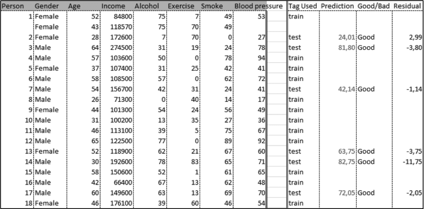Exhibit 08 – Training results example to forecast the bloody pressure where some data is used for testing the network results (Palisade Neural Tools software example)

Prediction Results

After the training, the model is ready to predict future results. The most relevant information that should be a focus of investigation is the contribution of each individual variable to the predicted results (Exhibit 09) and the reliability of the model (Exhibit 10).

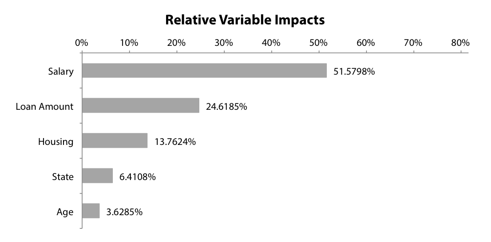Exhibit 09 – Example of Relative Variable impacts, demonstrating that the Salary variable is responsible for more than 50% of the impact in the dependent variable (Palisade Neural Tools software example)

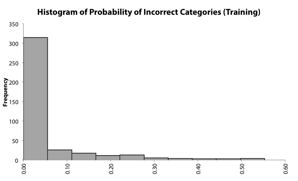Exhibit 10 – Example of histogram of Probability of Incorrect Categories showing a chance of 30% that 5% of the prediction can be wrong (Palisade Neural Tools software example)

It is important to highlight that one trained network that fails to get a reliable result in 30% of the cases is much more unreliable than another one that fails in only 1% of the cases.

Example of Cost Modeling using Artificial Neural Networks

In order to exemplify the process, a fictitious example was developed to predict the project management costs on historical data provided by 500 cases. The variables used are described in the Exhibit 11.

The profiles of the cases used for the training are presented at the Exhibit 12, 13, 14, 15 and 16 and the full dataset is presented in the Appendix.

Exhibit 12 – Distribution of cases by Location

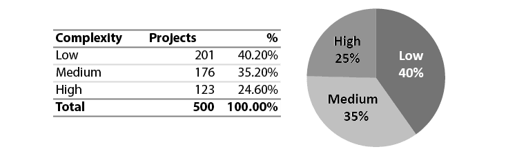Exhibit 13 – Distribution of cases by Complexity

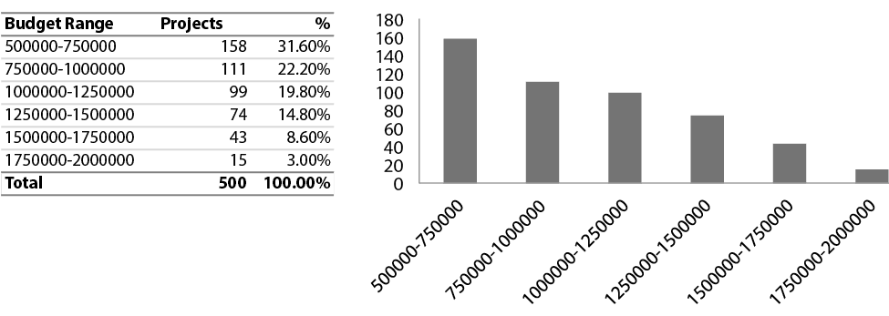Exhibit 14 – Distribution of cases by Project Budget

Exhibit 15 – Distribution of cases by Project Duration

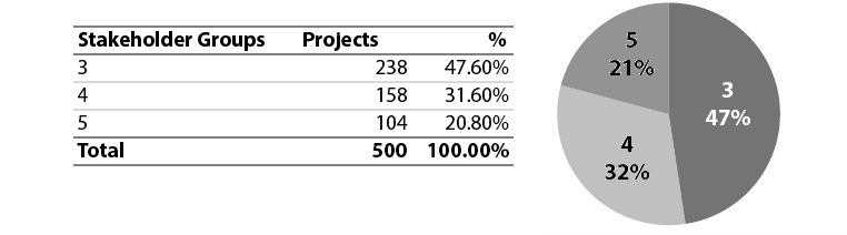Exhibit 16 – Distribution of cases by Relevant Stakeholder Groups

The training and the tests were executed using the software Palisade Neural Tools. The test was executed in 20% of the sample and a GRNN Numeric Predictor. The summary of the training of the ANN is presented at the Exhibit 17.

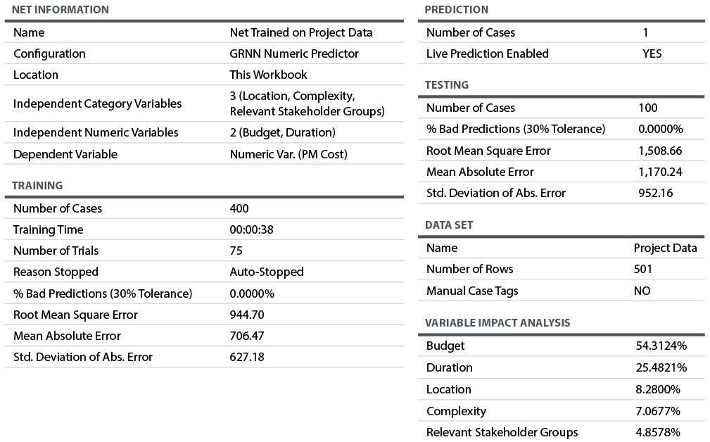Exhibit 17 – Palisade Neural Tools Summary Table

The relative impact of the five independent variables are described at the Exhibit 18, demonstrating that more than 50% of the impact in the Project Management cost is related to the project budget in this fictitious example.

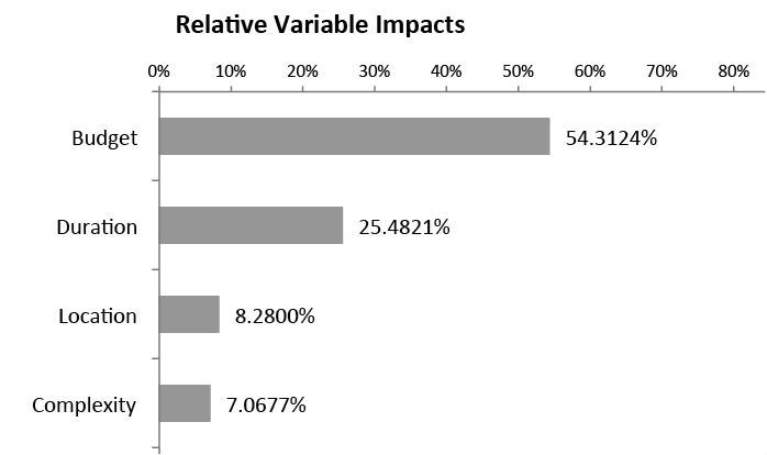Exhibit 18 – Relative Variable Impacts

The training and tests were used to predict the Project Management Cost of a fictitious project with the following variables

After running the simulation, the Project Management cost predictions based on the patterns in the known data is $24,344.75, approximately 3% of the project budget.

Conclusions

The use of Artificial Neural Networks can be a helpful tool to determine aspects of the project budget like the cost of project management, the estimated bid value of a supplier or the insurance cost of equipment. The Neural Networks allows some precise decision making process without an algorithm or a formula based process.

With the recent development of software tools, the calculation process becomes very simple and straightforward. However, the biggest challenge to produce reliable results lies in the quality of the known information. The whole process is based on actual results, and most of the time the most expensive and laborious part of the process is related to getting enough reliable data to train and test the process.

References

AIBINU, A. A., DASSANAYAKE, D. & THIEN, V. C. (2011). Use of Artificial Intelligence to Predict the Accuracy of Pretender Building Cost Estimate. Amsterdam: Management and Innovation for a Sustainable Built Environment.

ARAFA, M. & ALQEDRA, M. (2011). Early Stage Cost Estimation of Buildings Construction Projects using Artificial Neural Networks. Faisalabad: Journal of Artificial Intelligence.

BAILER-JONES, D & BAILER-JONES, C. (2002). Modeling data: Analogies in neural networks, simulated annealing and genetic algorithms. New York: Model-Based Reasoning: Science, Technology, Values/Kluwer Academic/Plenum Publishers.

BARTHA, P (2013). Analogy and Analogical Reasoning. Palo Alto: Stanford Center for the Study of Language and Information.

CHEUNG, V. & CANNONS, K. (2002). An Introduction to Neural Networks. Winnipeg, University of Manitoba.

INGRASSIA, S & MORLINI, I (2005). Neural Network Modeling for Small Datasets In Technometrics: Vol 47, n 3. Alexandria: American Statistical Association and the American Society for Quality

KOHONEN, T. (2014). MATLAB Implementations and Applications of the Self-Organizing Map. Helsinki: Aalto University, School of Science.

KRIESEL, D. (2005). A Brief Introduction to Neural Networks. Downloaded on 07/01/2015 at https://www.dkriesel.com/_media/science/neuronalenetze-en-zeta2-2col-dkrieselcom.pdf

MCKIM, R. A. (1993). Neural Network Applications for Project Management. Newtown Square: Project Management Journal.

SODIKOV, J. (2005). Cost Estimation of Highway Projects in Developing Countries: Artificial Neural Network Approach. Tokyo: Journal of the Eastern Asia Society for Transportation Studies, Vol. 6.

SPECHT, D. F. (2002). A General Regression Neural Network. New York, IEEE Transactions on Neural Networks, Vol 2, Issue 6.

SPITZIG, S. (2013). Analogy in Literature: Definition & Examples in SAT Prep: Help and Review. Link accessed on 06/30/2015: https://study.com/academy/lesson/analogy-in-literature-definition-examples-quiz.html

STERGIOUS, C & CIGANOS, D. (1996). Neural Networks in Surprise Journal Vol 4, n 11. London, Imperial College London.

SVOZIL, D, KVASNIČKA, V. & POSPÍCHAL, J. (1997). Introduction to multi-layer feed-forward neural networks In Chemometrics and Intelligent Laboratory Systems, Vol 39. Amsterdam, Elsevier Journals.